Success-counting dice pools: quadratic pool size ≈ linear fixed-die modifier

Last time, we looked at the mean, variance, and standard deviation of success-counting dice pools. Now, we are going to use these statistics to transform success-counting dice pools into a fixed-die system with similar probabilities.

Why transform into a fixed-die system?

Our first transformation into a fixed-die system was with keep-highest dice pools, and the reasoning there still applies. With other such transformations under our belt, including opposed keep-highest dice pools and step dice, we can compare all of these systems using this common basis. The purpose of this article is not to suggest that you should actually use the transformation in the game, it’s just to show a similarity in probabilities between two different systems.

At some point I will write an overview article for this technique with a more comprehensive motivation.

The “swinginess” paradox

Here’s another way of looking at it: What happens to the “swinginess” of a success-counting dice pool as the pool gets larger?

Some would say that it increases, because as you add more dice, the standard deviation of the number of successes increases.
Some would say that it decreases, referencing the law of large numbers.

The short answer is that “swinginess” is not a well-defined term, and so it’s no wonder that two different implied definitions come up with two different answers. The first defines it as the standard deviation of the number of successes as an absolute quantity, and the second defines it as the standard deviation relative to the mean number of successes. The former is proportional to the square root of the number of dice, and the latter is proportional to the inverse square root of the number of dice.

However, these are not the only choices. It’s easy to assume progression corresponds linearly to the pool size or target number of successes. But what if instead we had a nonlinear relationship between progression and pool size such that the standard deviation of the number of successes was equal to the rate of growth of the pool size? Then, no matter where you are in the progression, a standard deviation covers the same amount of progression.

This is what the transformation to a fixed-die system gives us.

1 standard deviation in the dice pool = 1 standard deviation in the fixed-die

In a fixed-die system, the dice that are rolled never change, and so their standard deviation never changes. Let the mean of the fixed-die dice be $\mu_a$ and the standard deviation be $\sigma_a$ . Let’s find a transformation from the success-counting dice pool size $A$ to the fixed-die modifier $a$ so that a difference of 1 standard deviation in the dice pool system produces a change of 1 standard deviation in the fixed-die system. Specifically, let’s require that the rate of change in the mean (i.e. average number of successes) of the dice pool $\mu_A$ with respect to standard deviations in the fixed-die system $a / \sigma_a$ is equal to the standard deviation in the dice pool system $\sigma_A$ :

$\sigma_a \frac{d \mu_A }{da} = \sigma_A$

Recall from last time that we can express the mean $\mu_A$ and standard deviation $\sigma_A$ of the entire pool in terms of the number of dice in the pool $A$ and the mean $\mu_1$ and standard deviation $\sigma_1$ of the individual dice:

$\mu_A = \mu_1 A$

$\sigma_A = \sigma_1 \sqrt{A}$

Substituting these in, we have:

$\sigma_a \mu_1 \frac{dA}{da} = \sigma_1 \sqrt{A}$

$\sigma_a \frac{\mu_1}{\sigma_1} \frac{ 1 }{\sqrt{A}} dA= da$

Integrating, we get:

$a = 2 \sigma_a \frac{\mu_1}{\sigma_1} \sqrt{A} = 2 \sigma_a \frac{\mu_A}{\sigma_A}$

$A = \left( \frac{\sigma_1}{\mu_1} \frac{a}{ 2\sigma_a } \right)^2$

A linearly increasing modifier in a fixed-die system thus corresponds to a quadratic success-counting pool size. While this grows faster than linearly, it is asymptotically less dramatic than a keep-highest dice pool with variable TN, where it takes a geometric number of dice to keep up with a linearly increasing fixed-die modifier.

Granularity

If we take the derivative of the fixed-die modifier with respect to the dice pool size, we can get an idea of the granularity.

$\frac{da}{dA} = \sigma_a \frac{\mu_1}{\sigma_1} \frac{1}{\sqrt{A}}$

A large such derivative means that each additional die corresponds to a large change in the fixed-die modifier and thus that the granularity is coarse. Since this derivative decreases with the size of the dice pool $A$ , the local granularity of the success-counting dice pool is coarse at low pool sizes and fine at high pool sizes. The fineness of the local granularity scales as the square root of the pool size, so if you quadruple the pool size, the local granularity becomes twice as fine.

Coefficient of variation

Beyond this, the ratio $\sigma_1 / \mu_1$ , sometimes called the coefficient of variation, scales the granularity of the dice pool system across the board. If it is large, the dice pool system will have fine granularity for a given pool size, and if it is small, the dice pool system will have coarse granularity for a given pool size. It’s easier to change the mean number of successes per die than the standard deviation, so a low chance of success per die tends to produce finer granularity and a high chance of success per die tends to produce coarser granularity.

Precomputed coefficients of variation can be found in this table.

Choosing a level of granularity

As always, finer granularity is not necessarily better, as it means you need a larger difference in pool size in order to produce a given change in probabilities. Dice pools follow a “Goldilocks principle”: too few dice, and you start to get noticeably non-converged behavior as we’ll see below; too many dice, and it starts to take too long to physically roll. This means there is only a limited range of comfortable dice pool sizes; the finer the granularity, the less progression that you can fit within this range.

Variable granularity

In my opinion, this is what the variable target numbers in Old World of Darkness should have meant (assuming we make use of multiple successes required; if only a single success is required, this is a keep-highest dice pool rather than a success-counting pool):

High TN = high coefficient of variation = fine granularity = outcome more dominated by luck
Low TN = low coefficient of variation = coarse granularity = outcome more dominated by stat

TN should not determine difficulty; the target number of successes should be determined after the TN to produce the desired level of difficulty. If you don’t want to make players do the math on the mean number of successes, you could consider using an opposed roll with the same TN on both sides, in which case the side with more dice obviously has the advantage.

This variable granularity is roughly analogous to how the recent Worlds without Number (a fixed-die system) uses 1d20 for attacks and 2d6 for skills. On the other hand, New World of Darkness decided that having two primary parameters was more trouble than it was worth, and moved to a primarily fixed-TN system with only the required number of successes varying most of the time.

Total number of successes

In a non-opposed roll, the player is seeking some target total number of successes. Let’s call this $T$ , its corresponding DC in the fixed-die system $t$ , and say that $t = a + \mu_a$ when the mean total result is equal to the total required, which will correspond to about 50% chance. This gives:

$T = \mu_1 A = \mu_1 \left( \frac{\sigma_1}{\mu_1} \frac{a}{ 2 \sigma_a } \right)^2 = \left( \frac{\sigma_1}{ \sqrt{\mu_1}} \frac{t - \mu_a }{ 2 \sigma_a } \right)^2$

$t = 2 \sigma_a \frac{\sqrt{\mu_1}}{\sigma_1} \sqrt{T} + \mu_a$

Margin of success

Like the other non-fixed-die systems we’ve seen, the margin of success in a success-counting dice pool depends on more than the chance of success; for a given chance of success, the margin of success will (in the limit) be scaled proportional to the standard deviation of the number of successes, which is

$\sigma_A = \sigma_1 \sqrt{A} = \frac{\sigma_1^2}{\mu_1} \frac{a}{ 2\sigma_a }$

This is a linear relationship with the fixed-die modifier $a$ . So, for example, if you have:

Damage proportional to the margin of success.
Constant typical hit chance.
Pool size increasing quadratically.
Hit points increasing linearly.

Then the average number of attacks needed to destroy a target will remain about constant.

On the other hand, if you are basing critical hits on a fixed margin of success, then you can expect the critical hit rate to increase with pool size even if the chance to hit is kept constant.

Granularity

Since the mean number of successes per die $\mu_1$ is typically less than 1, this means that the number of successes typically has coarser granularity than the size of the dice pool. This means that stats have finer granularity than difficulties, which you may regard as a positive.

What die is rolled in the fixed-die system?

From above, the number of successes is proportional to the fixed-die modifier:

$T \propto \left( t - \mu_a \right) ^2$

If we take a Taylor expansion around $t_0, T_0$ , we have:

$T - T_0 \propto 2 \left( t_0 - \mu_a \right) \left(t - t_0 \right) + \left(t - t_0 \right)^2$

with no following terms.

The standard deviation of the number of successes $\sigma$ is proportional to the square root of the mean number of successes $T_0$ :

$\sigma \propto \sqrt{T_0} \propto t_0 - \mu_a$

If we measure $T - T_0$ in terms of this standard deviation, we have

$\frac{T - T_0}{\sigma} \propto 2 \left(t - t_0 \right) + \frac{1}{ t_0 - \mu_a } \left(t - t_0 \right)^2$

As $t_0, T_0 \rightarrow \infty$ , the quadratic term goes to zero, and distance from the mean in the fixed-die system corresponds proportionally to distance from the mean in the dice pool system. Thus, in the limit of a large dice pool, the fixed-die system has the same type of distribution as the dice pool, namely a Gaussian.

How good are these approximations?

We made a several approximations along the way here:

The above linear relationship is only in the limit of a large dice pool.
The sum of the dice pool only converges to a Gaussian distribution in the limit of a large dice pool.
We approximated the number of successes as continuous. In reality, we can only have an integer number of successes.
Few dice also means a limited range of possible results.
The tiebreaking method may shift things towards one side or the other. The above formulas treat ties as neutral.

All of these approximations improve as the dice pool gets larger. Let’s visualize how these approximations converge. We’ll do this by computing a quasi-PMF for each dice pool size $A$ :

For every possible total number of successes $T$ , compute the chance of scoring that total.
Subtract 0.5 from $T$ if computing the CCDF, in order to give only half credit for ties.
From $A$ and $T$ , compute the fixed-die modifier $a$ and DC $t$ .
Plot the chance of scoring each total number of successes versus $x = t - a$ .
We will not normalize the areas below the curves in the still images. This allows us to read off the chances for particular outcomes directly, as well as visually separating the curves for each dice pool size.
We will normalize them for the videos.

As the pool size increases, this should increasingly resemble a Gaussian distribution.

Let’s look at a few examples, using $\mu_a = 0$ and $\sigma_a = 1$ , so each fixed-die point converges to one standard deviation.

Coin flip

First, here’s a d6 pool where each die is counted as 1 success on a 4+, as Burning Wheel:

Here’s the PMF in video form, normalized and plotted against an ideal Gaussian:

(You may want to try right-click →Loop.)

And the CCDF:

The convergence is considerably slower than in the case of fixed-die systems where the number of dice is fixed (per system). All but the first approximation listed above is shared between both cases, so that’s the one that makes the difference: while the dice pool eventually overcomes the non-constant standard deviation of the number of successes, it takes more dice to do so.

The left tail in particular is unfavorable to small dice pools. This is mostly because rolling 0 successes is both reasonably likely and also considered quite a bad result by the transformation. As the number of dice increases, the left side too starts to look like a Gaussian as desired.

Weighted coin flip

What if we change the threshold on each die? Here’s the same graph where a 5+ is needed for each die to count as a success, as Shadowrun 4e:

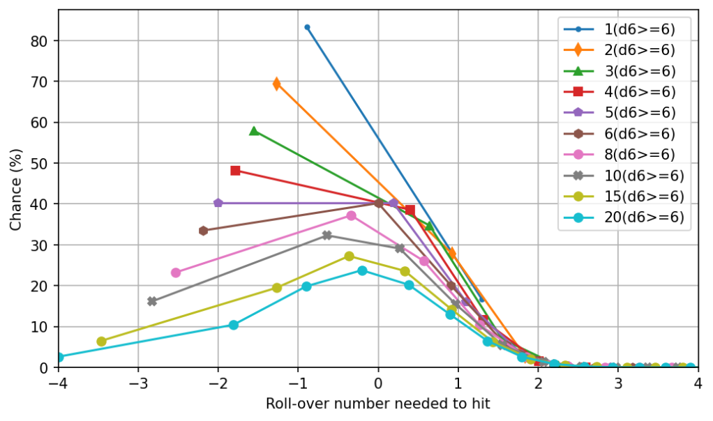
We can see that very low success chances slow the convergence to a Gaussian. On the other side, as with Burning Wheel shades, here’s success on 3+:

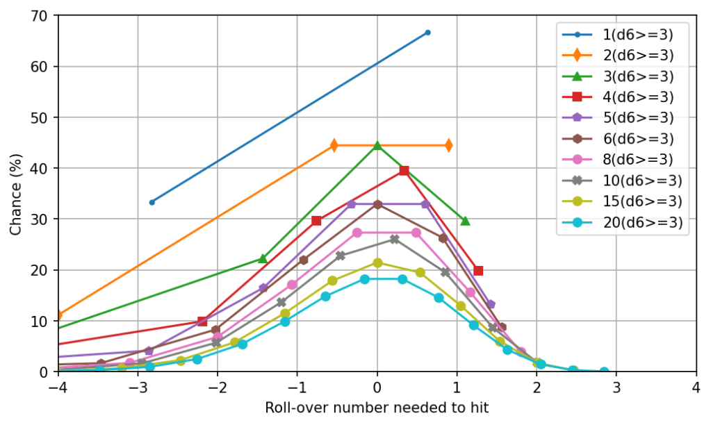
And on a 2+:

So very high success chances on each die also slows convergence to a Gaussian.

Double success on top face

Here’s another example, where the dice are those from Exalted 2e (d10s where 7+ is counted as 1 success and 10 as 2 successes):

To my eye, this converges to a Gaussian a bit faster to than the Burning Wheel die, though it is also more complicated.

Negative success on bottom face

d10s that succeed on a 7+ but subtract one success on 1s, as Old World of Darkness:

Exploding dice

An example with exploding dice: d10s that succeed on a 8+ and explode on 10s, as New World of Darkness:

Opposed

How about opposed rolls? If both sides roll $A$ dice each, then the total number of dice doubles and the standard deviation for the die pool increases by a factor $\sqrt{2}$ . On the other hand, if in the corresponding fixed-die system both sides roll, the standard deviation increases by the same factor there. So overall we can expect a Gaussian still, just with a larger standard deviation and finer granularity by a factor $\sqrt{2}$ .

Graphing opposed rolls is trickier since now there are two sides of dice involved. Here’s how we’ll do it:

Each series represents the number of dice for side $A$ .
The points in the series represent the number of dice for side $B$ , with the leftmost point in each series being $B = 0$ .
We’ll compute the chances of $A$ winning for each of these points. This produces a quasi-CCDF. Then we’ll produce a quasi-PMF by taking successive differences.
We’ll transform $A$ to $a$ using the formulas above, and transform $B$ to $b$ in the same way. The x-coordinate is the difference between the two sides $x = b - a$ .
Ties are broken by coin flip. I’m not necessarily recommending this tiebreaking system; I’m just using it as an example because it’s simple and neutral.

Here’s the result for Burning Wheel dice:

Again in video form, the PMF:

And the CCDF:

The convergence to a Gaussian is considerably faster than the non-opposed case past the first few dice. The non-opposed case needs a pool size of more than 50 dice to reach a maximum absolute difference in chance to hit of 1% compared to a perfect Gaussian. This opposed case requires just $A = 10$ dice to achieve the same. Here are some contributing factors:

Since the opposition $B$ is also rolling dice, this helps the curves converge more quickly in terms of $A$ , though in terms of total dice rolled this particular factor is about a wash. This does give you the option to reduce the number of dice rolled by half, i.e. about the same total dice split among both sides, which would about cancel out the increase in standard deviation and fineness of the granularity.
There’s always a nonzero chance for the underdog to win, regardless of the disparity in the pool sizes. This makes the right tail close to a Gaussian from the get-go. This isn’t true of the non-opposed case, where there’s a hard limit on what the underdog can achieve with simple TN-based dice. Additional rules such as explosions can get around this, but introduce additional complexity and rolling.

Of course, how these weigh with other factors such as aesthetics and speed of play is up to you.

Example transformation: Burning Wheel vs. Powered by the Apocalypse

Suppose we wanted to transform dice pool system where a 4+ on a d6 is a success (as Burning Wheel) to a 2d6 fixed-die system (as Powered by the Apocalypse). Again, I’m not advocating that you actually use such a transformation, this is just to give an example of how the transformation converges and how granularities might compare.

PbtA’s 2d6 is triangular, though this doesn’t actually make as much difference compared to a Gaussian as it may first appear. The mean is $\mu_a = 7$ , the variance is $\sigma_a^2 = 70/12$ , and the standard deviation is $\sigma_a \approx 2.415$ . 4+ on a d6 has $\sigma_A / \mu_A = 1$ . Using the formulas above, we find that $a \approx 4.83 \sqrt{A}$ , resulting in this table of correspondences:

BW pool size	BW successes needed	PbtA fixed-die modifier	PbtA fixed-die DC
0	0.0	0.0	7.0
1	0.5	4.8	11.8
2	1.0	6.8	13.8
3	1.5	8.4	15.4
4	2.0	9.7	16.7
5	2.5	10.8	17.8
6	3.0	11.8	18.8
7	3.5	12.8	19.8
8	4.0	13.7	20.7
9	4.5	14.5	21.5
10	5.0	15.3	22.3

Note how the dice pool has very coarse granularity at the low end and gets finer as the size of the pool increases, reaching parity with the fixed-die system (i.e. +1 die in the pool = +1 modifier in the fixed-die) at about 6 dice.

As with any fixed-die system, we can add or subtract a constant of our choice from all modifiers and DCs without producing any change in the probabilities. This allows us to shift the correspondences up and down, which will shall do forthwith.

The reverse transformation

As usual, the transformation works both ways. Modifiers in PbtA usually run from -1 to +3, so we’ll line that up with 5-9 dice in the pool so that each die is about equal to one point of modifier. This is equivalent to subtracting 11.8 from all the fixed-die modifiers and DCs in the table above.

“Winning” in PbtA corresponds to rolling the median or better at a +0, which we’ve equated to 6 dice in the pool, so we’ll look for 3 total successes there. “Winning at a cost” is 4 rows harder than that, or 5 total successes required. All in all, PbtA transformed to BW dice and rounded off to the nearest integer looks like this:

Your dice pool size is equal to your 6 + your PbtA modifier.
If you roll at least five 4+s , you win.
If you roll at least three 4+s, you win at a cost.
Otherwise, you lose.

Here are the probabilities:

PbtA bonus	BW dice	PbtA chance of 7+	BW chance of 3+ successes	PbtA chance of 11+	BW chance of 5+ successes
-1	5	41.7%	50.0%	2.8%	3.1%
0	6	58.3%	65.6%	8.3%	10.9%
1	7	72.2%	77.3%	16.7%	22.7%
2	8	83.3%	85.5%	27.8%	36.3%
3	9	91.7%	91.0%	41.7%	50.0%

I’d say that’s not too bad a match considering that these pool sizes are only moderately converged to a Gaussian, we used quite a bit of rounding, and we didn’t make any explicit adjustments for tiebreaking (though the roller winning ties in both cases roughly cancels each other out).

If we instead match a difference of two BW dice to every point of PbtA bonus, we can get much closer to convergence:

Your BW dice pool size is equal to your 24 + twice your PbtA modifier.
If you roll at least sixteen 4+s, you win.
If you roll at least twelve 4+s, you win at a cost.
Otherwise, you lose.

PbtA bonus	BW dice	PbtA chance of 7+	BW chance of 12+ successes	PbtA chance of 11+	BW chance of 16+ successes
-1	22	41.7%	41.6%	2.8%	2.6%
0	24	58.3%	58.1%	8.3%	7.6%
1	26	72.2%	72.1%	16.7%	16.3%
2	28	83.3%	82.8%	27.8%	28.6%
3	30	91.7%	90.0%	41.7%	42.8%

Again, I’m not recommending that you actually use this transformation. This is just to demonstrate the convergence of the transformation.

Conclusion

The major results of this article series are:

Success-counting dice—whether they use a simple target number on each die, count some faces as multiple or negative successes, or even explode—will converge to a Gaussian distribution as the size of the pool grows.
The mean number of success grows proportionally to the pool size, but the standard deviation grows only as the square root of the pool size.
A success-counting dice pool can be transformed into a fixed-die system with similar probabilities, with the approximation becoming increasingly close as the size of the pool increases.
- A linear amount of fixed-die modifier corresponds to a quadratic pool size.
- Likewise for fixed-die DC versus target number of successes.
- Even with the above nonlinear relationships, the corresponding fixed-die system still converges to a Gaussian distribution as the pool size increases, albeit more slowly.

Finally, although I did compute an expansive table of success-counting dice options and their statistics, I’d say: don’t underestimate the simple fixed target number! For a given complexity budget, the simpler the individual dice, the more dice you can “afford” to roll, and simply being able to roll larger pools comes with a host of benefits. As we’ve seen throughout this article, larger pools are closer to a Gaussian and their standard deviation is more consistent. Furthermore, a larger range of pool sizes allows for a higher progression ceiling and/or finer granularity, helping address some of the biggest challenges facing dice pools. And of course, rolling more dice feels great. When it comes to success-counting dice pools, quantity really is quality!

Appendices

Exploding dice and tails

While the quadratic relationship between the target number of successes and corresponding fixed-die DC slows convergence in most ways that we care about, there is one way in which it improves convergence. If I’m understanding this article correctly, the tail of the sum of geometric dice can be bounded by a geometric curve with any $\epsilon > 0$ longer half-life than an individual geometric die. Since it requires a quadratic number of successes to keep up with a linear increase in the corresponding fixed-die DC, the argument to that falloff is now quadratic and the long tail becomes Gaussian-like in the fixed-die equivalent.

Increasing standard deviation versus stat divergence

As noted before, the effect of each additional die decreases as the size of the pool increases. It could be argued that this could help counteract the divergence of raw stat values that often accumulates over time as characters pick this or that +1 to a stat and leave others untaken. I haven’t figured out to what extent I buy this argument.

Potential points against:

How much should stats be allowed to diverge in the first place?
This also affects situational modifiers, which I would prefer to maintain their effectiveness.

Integrating over a window

Our derivation was based on the standard deviation of the number of successes at a single point. I also considered integrating over some spread of fixed-die modifiers around the center, e.g.

$\displaystyle \tilde{A} = \frac{1}{2 \Delta a} \int_{a-\Delta a}^{a+\Delta a} \left( \frac{\sigma_1}{\mu_1} \frac{a}{ 2\sigma_a } \right)^2 da$

This comes out to adding a constant offset to the dice pool size $A$ in the formulas. This can help convergence in certain cases. However:

The purpose of this article is not to suggest that you should actually use the transformation, so fine optimization isn’t worth spending too much time on.
The improvement in convergence isn’t that large.
There’s no one offset that produces the best result in all cases.

Therefore I decided to stick with the simple version.

High Dice Roller

Success-counting dice pools: quadratic pool size ≈ linear fixed-die modifier

Why transform into a fixed-die system?

The “swinginess” paradox

1 standard deviation in the dice pool = 1 standard deviation in the fixed-die

Granularity

Coefficient of variation

Choosing a level of granularity

Variable granularity

Total number of successes

Margin of success

Granularity

What die is rolled in the fixed-die system?

How good are these approximations?

Coin flip

Weighted coin flip

Double success on top face

Negative success on bottom face

Exploding dice

Opposed

Example transformation: Burning Wheel vs. Powered by the Apocalypse

The reverse transformation

Conclusion

Appendices

Exploding dice and tails

Increasing standard deviation versus stat divergence

Integrating over a window

Leave a comment Cancel reply

Why transform into a fixed-die system?

The “swinginess” paradox

1 standard deviation in the dice pool = 1 standard deviation in the fixed-die

Granularity

Coefficient of variation

Choosing a level of granularity

Variable granularity

Total number of successes

Margin of success

Granularity

What die is rolled in the fixed-die system?

How good are these approximations?

Coin flip

Weighted coin flip

Double success on top face

Negative success on bottom face

Exploding dice

Opposed

Example transformation: Burning Wheel vs. Powered by the Apocalypse

The reverse transformation

Conclusion

Appendices

Exploding dice and tails

Increasing standard deviation versus stat divergence

Integrating over a window

Share this:

Related

Leave a comment Cancel reply