Previously, we looked at the maximum difference in chance to hit between uniform, triangular, and Gaussian distributions and found that it can be made smaller than a single face on a d20. But what if we are more concerned about the tails in particular?
Range and standard deviation
Range is often one of the first properties of dice that people think of. Conveniently, if you roll dice, the range is exactly times the range of an individual die.
As we add dice together, the shape of the distribution approaches a Gaussian by the central limit theorem. However, the width of the central “bell” is not determined by the range, but rather the standard deviation. Unlike the range, the standard deviation of the sum of dice is only times the standard deviation of a single die. Fortunately, this too is exact.
It is therefore useful to consider the ratio of the range to the standard deviation.1 From the above, we can conclude that the range / SD for the sum of dice is exactly times that of an individual die.
Versus a true Gaussian
What if we wanted to compare the sum of some dice to a true Gaussian? Unfortunately, we can’t compare the range, because a true Gaussian has infinite range.
What we can do is compute the chance that a Gaussian with the same standard deviation will generate a result outside the range of the sum of dice we are interested in. This is easily done by setting the standard score equal to half of range / SD and finding the corresponding percentile. Here’s a graphical example, comparing two d6s with a Gaussian with the same standard deviation:
The total of the two shaded areas is what we will compute for various sums of dice.
Sum of fair coin flips
We’ll look at two examples. First is the fair coin flip, or equivalently, counting 4+s on d6s. The range of a single coin is and the standard deviation is , so the range / SD of coins is . This results in the following table:
Number of coins
Range / SD
Chance of Gaussian rolling outside range
Rounded up
1
2.000
31.73%
1 in 3
2
2.828
15.73%
1 in 6
3
3.464
8.33%
1 in 12
4
4.000
4.55%
1 in 21
5
4.472
2.53%
1 in 39
6
4.899
1.43%
1 in 69
7
5.292
0.82%
1 in 122
8
5.657
0.47%
1 in 213
9
6.000
0.27%
1 in 370
10
6.325
0.16%
1 in 638
11
6.633
0.09%
1 in 1097
12
6.928
0.05%
1 in 1879
13
7.211
0.03%
1 in 3210
14
7.483
0.02%
1 in 5470
15
7.746
0.01%
1 in 9301
So, for example, the sum of nine coins spans six standard deviations end-to-end.
The chances are given for the Gaussian rolling off either end combined. Half of this will be above the range and half below.
Sum of d6s
What if we sum full d6s? The range of a d6 is 5 and the standard deviation is , so the range / SD of d6 is . In terms of range / SD, a d6 could be said to be worth coins. The table for d6s is:
nd6
Range / SD
Chance of Gaussian rolling outside range
Rounded up
1
2.928
14.32%
1 in 6
2
4.140
3.84%
1 in 26
3
5.071
1.12%
1 in 89
4
5.855
0.34%
1 in 292
5
6.547
0.11%
1 in 940
6
7.171
0.03%
1 in 2974
7
7.746
0.01%
1 in 9301
8
8.281
< 0.01%
1 in 28842
9
8.783
< 0.01%
1 in 88853
10
9.258
< 0.01%
1 in 272288
If we aim to cover about 95% of the probability of a Gaussian within the range, then 4 coins or 2d6 will do it. For about 99%, 7 coins or 3d6.
Other dice
In general, a standard die with faces has range / SD
Here’s a table:
Faces
Number of coins with same range / SD
2
1.00
4
1.80
6
2.14
8
2.33
10
2.45
12
2.54
20
2.71
Continuous
3.00
If we could create a continuous uniform distribution, each would be worth exactly 3 coins in terms of range / SD. Practically, since d6s are the most readily available and they’re already more than halfway to this theoretical maximum, I don’t think covering more of a Gaussian alone is a compelling reason to use larger dice. Of course, you might choose larger dice for other reasons, e.g. you want finer granularity without adding more dice.
1I considered calling this the studentized range; however, it appears that this term is exclusively used to refer to samples rather than known probability distributions.
Exploding dice (“acing” as Savage Worlds calls it) have tails that drop off like a geometric distribution. What would happen if we had step dice that actually followed a geometric distribution? Spoiler: it’s great in theory, but exploding dice don’t actually follow a geometric distribution well.
Non-opposed
An exploding die of size has an asymptotic half-life of .
For example, for an exploding d10, on average every ~3 points of DC halves the chance to succeed.
If the dice were perfectly geometric, the chance of success against a target number would be
As with keep-highest dice pools, we can take some logarithms to transform this into a modifier + fixed die system:
where is a half-life of our choosing (note that this is distinct from . This is a Gumbel distribution similar to what we got when we transformed keep-highest dice pools with variable target number into a fixed-die system, except in this case it’s a roll-under system rather than a roll-over system. As a reminder, here’s that Gumbel PMF:
In the roll-under case, the player is hoping that the die rolls to the left of the number needed to hit (usually their stat). As such, things are going to get very hard very quickly if their stat is low (left side), but their chance of missing only drops off slowly at high stat (right side). As usual for roll-under, this is the opposite to the roll-over case where the player adds the roll to their stat, and is looking to roll to the right of the number needed to hit.
The above is for a roll-over geometric step die system. If instead the geometric step die system were roll-under, it would correspond to a roll-over Gumbel + modifier system.
Summary table
Here’s a summary of values for standard die sizes:
Die size
Half-life
Inverse half-life
4
2.00
3.00
0.500
6
2.32
3.64
0.431
8
2.67
4.25
0.375
10
3.01
4.77
0.332
12
3.35
5.23
0.299
20
4.63
6.63
0.216
Opposed
As with keep-highest dice pools and Elo ratings, two opposed Gumbel distributions become a logistic distribution. Here’s the PMF for that again, along with exploding + standard dice that approximate them:
How well do exploding dice approximate a geometric distribution?
Unfortunately, exploding dice aren’t geometric, and as the dice get larger, their deviation from the geometric distribution gets increasingly severe. On a semilogy plot, the chance of hitting should slope down in a straight line with a steepness inversely proportional to . Here’s a plot (roller wins ties):
Note the logarithmic vertical scale.
However, the actual exploding dice look like this:
If the geometric distribution is like parachuting to the ground, a standard exploding die by itself is like falling off a tree and hitting every branch on the way down. The series for each die has periodic bumps, which become longer and larger the more faces the die has, and in fact, there are points at which each die performs worse than the next-smaller die. Here’s a plot of the ratio of the actual to the ideal (on a linear scale):
For opposed rolls, as the dice get larger, the behavior is increasingly dominated by the non-exploding part of the die, since only the highest single face explodes. Here’s a plot of the chance for the underdog to win against an opponent with twice their die size:
As the dice get larger, the probability of the underdog winning converges to 25%, the same as if the dice were not exploding.
Conclusion
Exploding dice have the same asymptotic falloff as a geometric distribution; if they followed a geometric distribution perfectly, they would correspond to a Gumbel (or logistic, if opposed) distribution in a die + modifier system.
However, their overall approximation of a geometric distribution is rather crude. In the case of Savage Worlds in particular, this is somewhat compensated for by the raise system, where beating the target by 4 gives extra effects. Even if the “better” die has a lower chance of succeeding, it will have a better chance of succeeding with a raise. In general, margin-of-success systems tend to help smooth out curves.
Appendices
The wild die
What about Savage World‘s Wild Die? Here’s the to-hit plot with the Wild Die included:
So mostly the Wild Die pushes the weaker dice up towards the stronger dice, effectively making the granularity more fine. However, most of the curves are still quite bumpy.
The Elo rating system was created by Arpad Elo to represent the relative skills between chess players. Since then, it has been used in other competitive activities from sports to tabletop games to video games.
Can Elo ratings be translated to stats in a tabletop RPG? The Elo model of the world is exactly the same as an opposed fixed-die system: each player’s performance follows some distribution around their rating, and the higher performer wins the match. So in fact such a translation is quite easy.
What’s the probability distribution?
It’s commonly assumed that the normal distribution is the most realistic distribution. Indeed, Elo’s original rating system assumed that each player’s performance is normally distributed. However, while some modern Elo systems still use the normal distribution (e.g. TrueSkill), most modern Elo systems instead use the logistic distribution. The logistic distribution has exponential tails rather than Gaussian tails, and thus assigns a greater chance for an underdog to pull off an upset.
This includes derivatives of Elo such as Glicko, which differ in terms of how they handle uncertainties in player skill, but whose model of performance is still logistic at their core. These differences usually aren’t a concern in RPG design, since we are simply assigning a true skill level to characters rather than trying to guess it from the outcome of matches.
The Elo formula
Given the ratings of two players and , the Elo system predicts the chance of player winning as:
The base of 10 and the divisor of 400 are arbitrary; changing them just rescales the ratings of the players. However, these are the most commonly-used values; when someone talks about “the” Elo rating system, they are most likely referring to this equation and these values.
Note that, just like modifiers in a fixed-die system, the absolute rating doesn’t matter—only the difference in ratings between two players.
Even for the same game, different Elo lists may have different starting ratings, different constants, and different players, so ratings in one list cannot be directly compared against ratings from another list.
A raffle where each side gets a number of tickets that grows exponentially with their rating. One ticket is drawn at random and its owner is the winner of the opposed roll. Every 400 points multiplies their tickets by a factor of 10. If we equate tickets in this raffle to Dragon Ball Power Levels, being “over 9000” would correspond to a difference of about +1300 Elo over a normal human with a Power Level of 5.1
An opposed keep-highest dice pool, where each side’s pool size grows exponentially with their rating. Every 400 points multiplies their pool size by a factor of 10. Ties are broken by discarding all dice that didn’t participate in the tie, and rerolling the rest.
An opposed fixed-die system, where each side rolls on a Gumbel distribution and adds their modifier. The Gumbel distribution is well-approximated by the sum of an exploding d10 plus another die of similar size; a d12 is the closest, while a d10 (possibly also exploding2) is not too far off either. Since for exploding d10s each 10 points of modifier makes a factor of 10 difference in the tail, 40 Elo rating is equal to 1 point of fixed-die modifier on these dice. Here’s a plot with ties broken by coin flip:
Converting real-life examples to fixed-die modifier
Here’s atable for chess derived from a 2004 distribution published by uschess.org. If we divide by 40 (as appropriate for exploding d10s), we get approximately the following:
According to this analysis, 220 Starcraft 2 MMR points is comparable to 100 Elo points, which means about 90 MMR per fixed-die modifier. If we apply that to this table at time of writing, we get approximately:
This is a narrower range than the previous examples, but note that this is confined to a single professional league. They estimated home-court advantage at 100 Elo points, or +2.5 fixed-die modifier with exploding d10s.
Compositing and de-compositing contests
An entire game (or match in the tennis example) may be longer than we want to resolve in a single roll in a RPG. If we consider a series of contests, what is the relationship between the Elo rating for the individual contests and for the entire series? Fortunately, one François Labelle has already done this analysis:
The logistic distribution experiences a constant multiplier to the Elo ratings when the players continue until one player’s total victories exceeds the other’s by a specified margin. That margin multiplies the effective difference between Elo ratings, e.g. win-by-two doubles the effective Elo difference, win-by-three triples it, and so forth.
The normal distribution experiences a near-constant multiplier when we hold a first-to- (or equivalently, best-of-) series of contests, where the effective difference between Elo ratings is scaled proportional to (though there is some convergence with involved).
Intuitively, for a single contest an underdog only needs to get lucky once to win, but in a series of contests they are less likely to get lucky enough times to win the entire series.
We can apply this in reverse to turn a single contest into a series of sub-contests. For example, if we think a contest (e.g. a debate, a battle, a crafting competition) is similar to a win-by-two series of sub-contests, then given a set of Elo ratings/fixed-die modifiers for the full contest we could divide the Elo ratings/fixed-die modifiers by two when trying to represent the individual sub-contests. Equivalently, we could instead double the number rolled on the dice, increasing their effect relative to the modifiers of the contestants.
The above calculations assume that the results of the sub-contests are independent; if they are correlated, then you could try a less aggressive scaling.
Conclusion
The Elo rating system’s model of performance is easily translated to physical dice. In fact, there are several possible rolling processes that fit the bill.
If the development of the Elo rating system is any clue, the logistic distribution is at least a plausible alternative to the normal distribution for modeling performance. The logistic distribution produces more outliers than the normal distribution, giving underdogs a better chance of pulling off an upset.
The effect of compositing several contests into a single super-contest or breaking up a single contest into several sub-contests can be modeled by multiplying or dividing all ratings by some factor.
Appendix: other dice options
10 is the roundest number to us humans, which is why we used exploding d10s as the running example. However, the granularity may be excessively fine for some games. For something with coarser granularity, I’d go with 2d((d6-1)!) by treating the “6” face on the die as an exploding 5. In this case, the asymptotic half-life is 1.934 and each point of modifier corresponds to 62.25 Elo. Here’s a plot:
Unfortunately, it’s difficult to come up with a good scheme with moderately more coarseness than this:
Two d6s per side with faces 0, 0, 0, 1, 1, 1-with-explosion. Problem: Too coarse.
Exploding d4s. Problems: d4s feel bad to roll, too many explosions slow down play.
Dividing the result of the die by 2. Problem: Not appreciably simpler than just accepting a finer granularity.
Custom dice. Problem: Physical investment is a big thing to ask.
One standard d10 per side that explodes on 5s rather than 10s. Problem: Not exploding on the highest face feels strange, and the peak of the PMF gets squashed too much.
As mentioned before, opposed keep-highest dice pools can also represent Elo ratings, but the number of dice can easily get out of hand. For example, +800 Elo would correspond to multiplying the pool size by a hundred! For a high stat ceiling, we would need to come up with some sort of pool reduction scheme to make this feasible. I’m considering the idea of trading dice for free explosions, but so far I haven’t come up with a scheme I’m satisfied with. De-compositing contests as above lowers the scale of Elo ratings and thus the growth of pool sizes, so this could be another strategy.
1Differences in Power Levels in canon are more impactful than in this raffle model. For example, the article states that
In order for someone to be able to take attacks from a foe without taking any damage, they must possess twice the power of their foe. […] In general, if one has a higher power level than one’s opponent, then they can defeat the one with the weaker power level. For example, “Person A” has a fighting power of 10,000 and “Person B” has a fighting power of 5,000. “Person A” can most certainly defeat “Person B”.
In contrast, under the raffle model, having twice the tickets only gives a 2/3 chance of winning. So Power Level = raffle tickets cannot really be considered a good direct representation of the television show canon. Then again, giving the underdog more of a chance is probably more appropriate for a game.
2The sum of multiple geometric distributions is a negative binomial distribution. While adding geometric distributions together makes the tail fall off more slowly asymptotically than a single geometric distribution with the same half-life, a single geometric distribution with even a slightly longer half-life will fall off even more slowly.
Last time, we looked at the mean, variance, and standard deviation of success-counting dice pools. Now, we are going to use these statistics to transform success-counting dice pools into a fixed-die system with similar probabilities.
Why transform into a fixed-die system?
Our first transformation into a fixed-die system was with keep-highest dice pools, and the reasoning there still applies. With other such transformations under our belt, including opposed keep-highest dice pools and step dice, we can compare all of these systems using this common basis. The purpose of this article is not to suggest that you should actually use the transformation in the game, it’s just to show a similarity in probabilities between two different systems.
At some point I will write an overview article for this technique with a more comprehensive motivation.
The “swinginess” paradox
Here’s another way of looking at it: What happens to the “swinginess” of a success-counting dice pool as the pool gets larger?
Some would say that it increases, because as you add more dice, the standard deviation of the number of successes increases.
The short answer is that “swinginess” is not a well-defined term, and so it’s no wonder that two different implied definitions come up with two different answers. The first defines it as the standard deviation of the number of successes as an absolute quantity, and the second defines it as the standard deviation relative to the mean number of successes. The former is proportional to the square root of the number of dice, and the latter is proportional to the inverse square root of the number of dice.
However, these are not the only choices. It’s easy to assume progression corresponds linearly to the pool size or target number of successes. But what if instead we had a nonlinear relationship between progression and pool size such that the standard deviation of the number of successes was equal to the rate of growth of the pool size? Then, no matter where you are in the progression, a standard deviation covers the same amount of progression.
This is what the transformation to a fixed-die system gives us.
1 standard deviation in the dice pool = 1 standard deviation in the fixed-die
In a fixed-die system, the dice that are rolled never change, and so their standard deviation never changes. Let the mean of the fixed-die dice be and the standard deviation be . Let’s find a transformation from the success-counting dice pool size to the fixed-die modifier so that a difference of 1 standard deviation in the dice pool system produces a change of 1 standard deviation in the fixed-die system. Specifically, let’s require that the rate of change in the mean (i.e. average number of successes) of the dice pool with respect to standard deviations in the fixed-die system is equal to the standard deviation in the dice pool system :
Recall from last time that we can express the mean and standard deviation of the entire pool in terms of the number of dice in the pool and the mean and standard deviation of the individual dice:
Substituting these in, we have:
Integrating, we get:
A linearly increasing modifier in a fixed-die system thus corresponds to a quadratic success-counting pool size. While this grows faster than linearly, it is asymptotically less dramatic than a keep-highest dice pool with variable TN, where it takes a geometric number of dice to keep up with a linearly increasing fixed-die modifier.
Granularity
If we take the derivative of the fixed-die modifier with respect to the dice pool size, we can get an idea of the granularity.
A large such derivative means that each additional die corresponds to a large change in the fixed-die modifier and thus that the granularity is coarse. Since this derivative decreases with the size of the dice pool , the local granularity of the success-counting dice pool is coarse at low pool sizes and fine at high pool sizes. The fineness of the local granularity scales as the square root of the pool size, so if you quadruple the pool size, the local granularity becomes twice as fine.
Coefficient of variation
Beyond this, the ratio , sometimes called the coefficient of variation, scales the granularity of the dice pool system across the board. If it is large, the dice pool system will have fine granularity for a given pool size, and if it is small, the dice pool system will have coarse granularity for a given pool size. It’s easier to change the mean number of successes per die than the standard deviation, so a low chance of success per die tends to produce finer granularity and a high chance of success per die tends to produce coarser granularity.
Precomputed coefficients of variation can be found in this table.
Choosing a level of granularity
As always, finer granularity is not necessarily better, as it means you need a larger difference in pool size in order to produce a given change in probabilities. Dice pools follow a “Goldilocks principle”: too few dice, and you start to get noticeably non-converged behavior as we’ll see below; too many dice, and it starts to take too long to physically roll. This means there is only a limited range of comfortable dice pool sizes; the finer the granularity, the less progression that you can fit within this range.
Variable granularity
In my opinion, this is what the variable target numbers in Old World of Darkness should have meant (assuming we make use of multiple successes required; if only a single success is required, this is a keep-highest dice pool rather than a success-counting pool):
High TN = high coefficient of variation = fine granularity = outcome more dominated by luck
Low TN = low coefficient of variation = coarse granularity = outcome more dominated by stat
TN should not determine difficulty; the target number of successes should be determined after the TN to produce the desired level of difficulty. If you don’t want to make players do the math on the mean number of successes, you could consider using an opposed roll with the same TN on both sides, in which case the side with more dice obviously has the advantage.
This variable granularity is roughly analogous to how the recent Worlds without Number (a fixed-die system) uses 1d20 for attacks and 2d6 for skills. On the other hand, New World of Darkness decided that having two primary parameters was more trouble than it was worth, and moved to a primarily fixed-TN system with only the required number of successes varying most of the time.
Total number of successes
In a non-opposed roll, the player is seeking some target total number of successes. Let’s call this , its corresponding DC in the fixed-die system , and say that when the mean total result is equal to the total required, which will correspond to about 50% chance. This gives:
Margin of success
Like the other non-fixed-die systems we’ve seen, the margin of success in a success-counting dice pool depends on more than the chance of success; for a given chance of success, the margin of success will (in the limit) be scaled proportional to the standard deviation of the number of successes, which is
This is a linear relationship with the fixed-die modifier . So, for example, if you have:
Damage proportional to the margin of success.
Constant typical hit chance.
Pool size increasing quadratically.
Hit points increasing linearly.
Then the average number of attacks needed to destroy a target will remain about constant.
On the other hand, if you are basing critical hits on a fixed margin of success, then you can expect the critical hit rate to increase with pool size even if the chance to hit is kept constant.
Granularity
Since the mean number of successes per die is typically less than 1, this means that the number of successes typically has coarser granularity than the size of the dice pool. This means that stats have finer granularity than difficulties, which you may regard as a positive.
What die is rolled in the fixed-die system?
From above, the number of successes is proportional to the fixed-die modifier:
If we take a Taylor expansion around , we have:
with no following terms.
The standard deviation of the number of successes is proportional to the square root of the mean number of successes :
If we measure in terms of this standard deviation, we have
As , the quadratic term goes to zero, and distance from the mean in the fixed-die system corresponds proportionally to distance from the mean in the dice pool system. Thus, in the limit of a large dice pool, the fixed-die system has the same type of distribution as the dice pool, namely a Gaussian.
How good are these approximations?
We made a several approximations along the way here:
The above linear relationship is only in the limit of a large dice pool.
The sum of the dice pool only converges to a Gaussian distribution in the limit of a large dice pool.
We approximated the number of successes as continuous. In reality, we can only have an integer number of successes.
Few dice also means a limited range of possible results.
The tiebreaking method may shift things towards one side or the other. The above formulas treat ties as neutral.
All of these approximations improve as the dice pool gets larger. Let’s visualize how these approximations converge. We’ll do this by computing a quasi-PMF for each dice pool size :
For every possible total number of successes , compute the chance of scoring that total.
Subtract 0.5 from if computing the CCDF, in order to give only half credit for ties.
From and , compute the fixed-die modifier and DC .
Plot the chance of scoring each total number of successes versus .
We will not normalize the areas below the curves in the still images. This allows us to read off the chances for particular outcomes directly, as well as visually separating the curves for each dice pool size.
We will normalize them for the videos.
As the pool size increases, this should increasingly resemble a Gaussian distribution.
Let’s look at a few examples, using and , so each fixed-die point converges to one standard deviation.
Coin flip
First, here’s a d6 pool where each die is counted as 1 success on a 4+, as Burning Wheel:
Here’s the PMF in video form, normalized and plotted against an ideal Gaussian:
(You may want to try right-click →Loop.)
And the CCDF:
The convergence is considerably slower than in the case of fixed-die systems where the number of dice is fixed (per system). All but the first approximation listed above is shared between both cases, so that’s the one that makes the difference: while the dice pool eventually overcomes the non-constant standard deviation of the number of successes, it takes more dice to do so.
The left tail in particular is unfavorable to small dice pools. This is mostly because rolling 0 successes is both reasonably likely and also considered quite a bad result by the transformation. As the number of dice increases, the left side too starts to look like a Gaussian as desired.
Weighted coin flip
What if we change the threshold on each die? Here’s the same graph where a 5+ is needed for each die to count as a success, as Shadowrun 4e:
And a 6 needed for a success:
We can see that very low success chances slow the convergence to a Gaussian. On the other side, as with Burning Wheel shades, here’s success on 3+:
And on a 2+:
So very high success chances on each die also slows convergence to a Gaussian.
Double success on top face
Here’s another example, where the dice are those from Exalted 2e (d10s where 7+ is counted as 1 success and 10 as 2 successes):
To my eye, this converges to a Gaussian a bit faster to than the Burning Wheel die, though it is also more complicated.
Negative success on bottom face
d10s that succeed on a 7+ but subtract one success on 1s, as Old World of Darkness:
Exploding dice
An example with exploding dice: d10s that succeed on a 8+ and explode on 10s, as New World of Darkness:
Opposed
How about opposed rolls? If both sides roll dice each, then the total number of dice doubles and the standard deviation for the die pool increases by a factor . On the other hand, if in the corresponding fixed-die system both sides roll, the standard deviation increases by the same factor there. So overall we can expect a Gaussian still, just with a larger standard deviation and finer granularity by a factor .
Graphing opposed rolls is trickier since now there are two sides of dice involved. Here’s how we’ll do it:
Each series represents the number of dice for side .
The points in the series represent the number of dice for side , with the leftmost point in each series being .
We’ll compute the chances of winning for each of these points. This produces a quasi-CCDF. Then we’ll produce a quasi-PMF by taking successive differences.
We’ll transform to using the formulas above, and transform to in the same way. The x-coordinate is the difference between the two sides .
Ties are broken by coin flip. I’m not necessarily recommending this tiebreaking system; I’m just using it as an example because it’s simple and neutral.
Here’s the result for Burning Wheel dice:
Again in video form, the PMF:
And the CCDF:
The convergence to a Gaussian is considerably faster than the non-opposed case past the first few dice. The non-opposed case needs a pool size of more than 50 dice to reach a maximum absolute difference in chance to hit of 1% compared to a perfect Gaussian. This opposed case requires just dice to achieve the same. Here are some contributing factors:
Since the opposition is also rolling dice, this helps the curves converge more quickly in terms of , though in terms of total dice rolled this particular factor is about a wash. This does give you the option to reduce the number of dice rolled by half, i.e. about the same total dice split among both sides, which would about cancel out the increase in standard deviation and fineness of the granularity.
There’s always a nonzero chance for the underdog to win, regardless of the disparity in the pool sizes. This makes the right tail close to a Gaussian from the get-go. This isn’t true of the non-opposed case, where there’s a hard limit on what the underdog can achieve with simple TN-based dice. Additional rules such as explosions can get around this, but introduce additional complexity and rolling.
Of course, how these weigh with other factors such as aesthetics and speed of play is up to you.
Example transformation: Burning Wheel vs. Powered by the Apocalypse
Suppose we wanted to transform dice pool system where a 4+ on a d6 is a success (as Burning Wheel) to a 2d6 fixed-die system (as Powered by the Apocalypse). Again, I’m not advocating that you actually use such a transformation, this is just to give an example of how the transformation converges and how granularities might compare.
Note how the dice pool has very coarse granularity at the low end and gets finer as the size of the pool increases, reaching parity with the fixed-die system (i.e. +1 die in the pool = +1 modifier in the fixed-die) at about 6 dice.
As with any fixed-die system, we can add or subtract a constant of our choice from all modifiers and DCs without producing any change in the probabilities. This allows us to shift the correspondences up and down, which will shall do forthwith.
The reverse transformation
As usual, the transformation works both ways. Modifiers in PbtA usually run from -1 to +3, so we’ll line that up with 5-9 dice in the pool so that each die is about equal to one point of modifier. This is equivalent to subtracting 11.8 from all the fixed-die modifiers and DCs in the table above.
“Winning” in PbtA corresponds to rolling the median or better at a +0, which we’ve equated to 6 dice in the pool, so we’ll look for 3 total successes there. “Winning at a cost” is 4 rows harder than that, or 5 total successes required. All in all, PbtA transformed to BW dice and rounded off to the nearest integer looks like this:
Your dice pool size is equal to your 6 + your PbtA modifier.
If you roll at least five 4+s , you win.
If you roll at least three 4+s, you win at a cost.
Otherwise, you lose.
Here are the probabilities:
PbtA bonus
BW dice
PbtA chance of 7+
BW chance of 3+ successes
PbtA chance of 11+
BW chance of 5+ successes
-1
5
41.7%
50.0%
2.8%
3.1%
0
6
58.3%
65.6%
8.3%
10.9%
1
7
72.2%
77.3%
16.7%
22.7%
2
8
83.3%
85.5%
27.8%
36.3%
3
9
91.7%
91.0%
41.7%
50.0%
I’d say that’s not too bad a match considering that these pool sizes are only moderately converged to a Gaussian, we used quite a bit of rounding, and we didn’t make any explicit adjustments for tiebreaking (though the roller winning ties in both cases roughly cancels each other out).
If we instead match a difference of two BW dice to every point of PbtA bonus, we can get much closer to convergence:
Your BW dice pool size is equal to your 24 + twice your PbtA modifier.
If you roll at least sixteen 4+s, you win.
If you roll at least twelve 4+s, you win at a cost.
Otherwise, you lose.
PbtA bonus
BW dice
PbtA chance of 7+
BW chance of 12+ successes
PbtA chance of 11+
BW chance of 16+ successes
-1
22
41.7%
41.6%
2.8%
2.6%
0
24
58.3%
58.1%
8.3%
7.6%
1
26
72.2%
72.1%
16.7%
16.3%
2
28
83.3%
82.8%
27.8%
28.6%
3
30
91.7%
90.0%
41.7%
42.8%
Again, I’m not recommending that you actually use this transformation. This is just to demonstrate the convergence of the transformation.
Conclusion
The major results of this article series are:
Success-counting dice—whether they use a simple target number on each die, count some faces as multiple or negative successes, or even explode—will converge to a Gaussian distribution as the size of the pool grows.
The mean number of success grows proportionally to the pool size, but the standard deviation grows only as the square root of the pool size.
A success-counting dice pool can be transformed into a fixed-die system with similar probabilities, with the approximation becoming increasingly close as the size of the pool increases.
A linear amount of fixed-die modifier corresponds to a quadratic pool size.
Likewise for fixed-die DC versus target number of successes.
Even with the above nonlinear relationships, the corresponding fixed-die system still converges to a Gaussian distribution as the pool size increases, albeit more slowly.
Finally, although I did compute an expansive table of success-counting dice options and their statistics, I’d say: don’t underestimate the simple fixed target number! For a given complexity budget, the simpler the individual dice, the more dice you can “afford” to roll, and simply being able to roll larger pools comes with a host of benefits. As we’ve seen throughout this article, larger pools are closer to a Gaussian and their standard deviation is more consistent. Furthermore, a larger range of pool sizes allows for a higher progression ceiling and/or finer granularity, helping address some of the biggest challenges facing dice pools. And of course, rolling more dice feels great. When it comes to success-counting dice pools, quantity really is quality!
Appendices
Exploding dice and tails
While the quadratic relationship between the target number of successes and corresponding fixed-die DC slows convergence in most ways that we care about, there is one way in which it improves convergence. If I’m understanding this article correctly, the tail of the sum of geometric dice can be bounded by a geometric curve with any longer half-life than an individual geometric die. Since it requires a quadratic number of successes to keep up with a linear increase in the corresponding fixed-die DC, the argument to that falloff is now quadratic and the long tail becomes Gaussian-like in the fixed-die equivalent.
Increasing standard deviation versus stat divergence
As noted before, the effect of each additional die decreases as the size of the pool increases. It could be argued that this could help counteract the divergence of raw stat values that often accumulates over time as characters pick this or that +1 to a stat and leave others untaken. I haven’t figured out to what extent I buy this argument.
Potential points against:
How much should stats be allowed to diverge in the first place?
This also affects situational modifiers, which I would prefer to maintain their effectiveness.
Integrating over a window
Our derivation was based on the standard deviation of the number of successes at a single point. I also considered integrating over some spread of fixed-die modifiers around the center, e.g.
This comes out to adding a constant offset to the dice pool size in the formulas. This can help convergence in certain cases. However:
The purpose of this article is not to suggest that you should actually use the transformation, so fine optimization isn’t worth spending too much time on.
The improvement in convergence isn’t that large.
There’s no one offset that produces the best result in all cases.
Therefore I decided to stick with the simple version.
It’s well-known that as you sum more and more standard dice together, the shape approaches a Gaussian distribution. But how much difference does the number of dice actually make?
Single d20 vs. Gaussian
First, we’ll compare a single d20 to a Gaussian. Since a Gaussian is a continuous distribution, we’ll discretize it by rounding all values to the nearest integer, which for a d20 is still plenty fine granularity.
Matching mean and standard deviation
The mean of a d20 is and its standard deviation is .
3d6 and 2d10 are often given as examples of how “the bell curve clusters results more towards the center compared to 1d20”. However, 1d20 has nearly twice the standard deviation of 3d6 (), and still nearly half again as much as 2d10 (). So in these cases, the clustering is mostly because of the smaller standard deviation rather than the inherent shape of the Gaussian.
Presumably these comparisons are made on the basis that they have the same range… except that they don’t have the same range (3d6 only runs from 3-18 and 2d10 from 2-20, rather than 1-20). Furthermore, a Gaussian has infinite range, which cannot be matched by any sum of a finite number of standard dice with any finite scaling. So matching the range of a Gaussian is not even a well-formed comparison. The most that could be said is that using multiple dice allows you to maintain the same range of what is possible to happen (even if the chances towards the ends may become arbitrarily small) while weighting results towards the middle.
Matching the standard deviation allows a well-formed comparison to a Gaussian. Here’s the PMF:
And the CCDF (chance to hit):
The peak of the Gaussian’s PMF has a height of about 6.9%, which is just under 1.4 times the chance of rolling any particular number of a d20.
The maximum absolute difference in chance to hit1 happens at a 16 (or symmetrically, 6) needed to hit. The d20 has a 25% chance to hit, while the Gaussian has a 19.29% chance to hit, a difference of 5.71% absolute chance.
The maximum relative difference in chance to hit in favor of the uniform distribution happens a point further out, where the uniform distribution delivers 1.34 times the hits of the Gaussian. (The ratio in the opposite direction is of course infinite once we go past the end of the d20.)
In terms of the chance to hit (or miss), the Gaussian’s tail becomes thicker than the uniform distribution only at a 20 (or 2) needed to hit or beyond. At this point, the Gaussian’s chance to hit is 5.93%, which is not a part of the curve you probably want to be using regularly. The chance of rolling above 20 is 4.14%.
So with the same standard deviation, there is a sense in which the Gaussian does cluster more towards the center, but by barely more than a single face on a d20 at most.
This is an example of how the difference in the PMF can look much more dramatic than the difference in chances to hit. This is because the chances to hit are derived from integrating the PMF, which can smooth out sharp areas.
Matching the 50th percentile
What if we matched the height of the PMF at the 50th percentile instead?2 This happens at around . This gives us the following PMF:
And the corresponding CCDF (chance to hit):
Now the CCDF curve lines up at the 50th percentile. Meanwhile, at the tail, the chance for the Gaussian to roll greater than a 20 is 10.56%, more than twice what it was when we matched the standard deviations.
The main effect in this case is to lengthen the tails beyond what is achievable by the d20, as we saw in our previous series about effective hit points in the tail. I consider this to be the most important aspect of a Gaussian compared to a uniform distribution—not clustering.
In fact, if we choose in order to minimize the largest absolute difference in chance to hit, we get an intermediate value for the standard deviation producing a maximum absolute difference in chance to hit of 4.8%. That’s less than a single full face on a d20. This standard deviation is approximately equal to 3d12 (AnyDice).
Margin of success
What the standard deviation does do pretty well is matching linear margins of success. Here the matched 50th percentile PMF has significantly higher mean margins of success for the Gaussian (counting misses as 0):
While the matched standard deviation is a close fit:
Also, the mean and standard deviation are always good ways of comparing two Gaussians, since a Gaussian is completely defined by these two parameters.
Opposed d20 vs. Gaussian
The sum or difference of two of the same standard die produces a triangular distribution. To make things truly symmetric, we’ll break ties by coin flip. Including the coin flip, the standard deviation is . Again, we’ll compare this to a Gaussian with the same standard deviation. First, the PMF:
And the CCDF (chance for underdog to win):
The peak of the Gaussian is 4.9%, virtually indistinguishable from the triangular. So this time there’s not much distinction between matching the standard deviation and matching the height of the PMF at the 50th percentile.
The maximum absolute difference in chance to win happens at a modifier disparity of 8. The triangular has a 18% chance of the underdog winning, while the Gaussian has a 16.37% chance of the underdog winning, a difference of 1.63%. That’s less than a third of a single face on a single d20.
The maximum relative difference in chance for the underdog in favor of the triangular distribution happens at a difference in modifiers of 11, where the triangular distribution delivers 1.14 times the wins for the underdog compared to the Gaussian.
The triangular’s chance for the underdog falls under the Gaussian’s starting at a difference in modifiers of 15. Here the chance for the underdog to win is just under 1 in 30. In Dungeons & Dragons 5th Edition, it takes a tarrasque versus a frog in a Strength check to produce this level of disparity.
Just 0.72% of rolls of the Gaussian are beyond each end of the triangular’s range. So while the Gaussian technically has an infinitely long tail, the chances of actually exceeding the end of the triangular’s tail is quite small.
Even the mean margin of success plot is very close:
So two of the same die is already most of the way to a Gaussian.
Mixed die sizes
Note that this mostly applies when the dice the same size or at least close to it. With heavily lopsided die sizes (e.g. d20 + d6), don’t expect anything more than rounding off the extreme ends, which most systems try to use less often anyways. Unless you prefer the aesthetic of the extra die, you might just use a flat modifier instead for simplicity.
Here are some example CCDFs:
Success-counting
The d20 is a fairly large die; how well do very small dice follow the Gaussian? Let’s look at counting 4+s on a d6 dice pool, which is equivalent to counting heads on coin flips. Since we are now comparing several different pool sizes, we’ll normalize according to the standard deviation and compare it to a continuous Gaussian. Here are the PMFs:
And the CCDFs:
(You may want to try right-click → Loop.)
The maximum absolute difference in chance to hit versus a discretized Gaussian with the same standard deviation drops below 1% at a pool size of just 4 coins. So the main differences are the coarse granularity and the range of possible results, not the overall shape of the CCDF.
Conclusion
Standard deviation isn’t always a great statistic for binary hit/miss. Alternatives include median absolute deviation, the height of the PMF at some reference percentile, and the maximum absolute difference in chance to hit1, depending on what exactly you’re trying to achieve.
Standard deviation does work perfectly for Gaussians and pretty well for linear margins of success.
With binary hit/miss, it’s possible to tune the standard deviation of a Gaussian so that the absolute difference in chance to hit compared to a d20 never reaches a full single face (5%).
The sum or difference of just two of the same standard die (a triangular distribution) is already most of the way to a Gaussian. More dice mostly extends the tails with extra possible but increasingly improbable rolls.
Even counting successes on coin flips converges to a Gaussian quickly. The major differences are the coarse granularity and the range of possible results, not the overall shape of the CCDF.
Overall, I’d say the main difference between a uniform, triangular, and Gaussian is whether the tails have a hard cutoff (uniform) versus a smooth (but still fairly steep) dropoff, and how far the range of improbable but technically possible rolls extends. Other than this, the probabilities are close enough that they should only be a secondary concern. Two standard dice should be plenty for all but the most discerning.
1 This is equivalent to the Kolmogorov-Smirnov statistic, though this seems to be an atypical application of the concept.
2 As usual, you don’t have to pick 50% exactly; if e.g. your system is expected to operate around a 60% typical chance to hit you could use that instead. Note though that this may also require using a different mean for the two distributions in order to get their CCDFs to match up horizontally at that percentile.
In this series, we’ll analyze success-counting dice pools. This is where the player rolls a pool of dice and counts the number that meet pass a specified threshold, with the size of the dice pool varying. Each die that does so is called a success in the well-known World of Darkness games. This nomenclature can unfortunately be confusing, but I’m not going to fight precedent here.
More than one success per die
Some variants on success-counting allow outcomes other than zero or one success per die. Here are some examples:
Exalted 2e where a 10 counts as 2 successes.
Classic World of Darkness where a 1 counts as a negative success.
New World of Darkness where a 10 explodes, allowing the player to roll an additional die.
D6 System where entire standard d6s are added together, thus effectively generating 1 to 6 “successes” per die.
As different as these may seem, they can all be analyzed using similar techniques. Of course, this doesn’t mean they play out the same at the table. In particular, counting is considerably easier per-die than adding standard dice.
The central limit theorem
The central limit theorem says that, as long as the dice in the pool have finite variance, the shape of the curve will converge to a normal distribution as the pool gets bigger. This is also known as a Gaussian distribution or informally as a bell curve. The choice of dice will affect how quickly this happens as we add dice—for example, looking for 6s on d6s will converge more slowly than looking for 4+s—but it will happen eventually. A Gaussian distribution is completely defined by its mean and variance (or standard deviation), so as the pool gets bigger, these become increasingly good descriptions of the curve.
If you’re planning to use dice pools that are large enough to achieve a Gaussian shape, you might as well choose something easy to use. Choosing a simple fraction for the mean such as 1/2 or 1/3 will make it easy for players to tell how many dice they should expect to need to have about a 50% chance of hitting a target total number of successes.
In a follow-up article, we’ll see how this convergence process looks for several types of dice.
Mean and variance “stack” additively
Conveniently, both the mean and variance of the sum of a set of dice “stack” additively: to find the mean and variance of the pool’s total, just sum up the means and variances of the individual dice. When all the dice are the same, as we are assuming here, it’s even easier: just multiply the mean and variance of a single die by the number of dice. Symbolically, if you have dice, where each of which has individual mean and variance , then the mean and variance of their sum are
The standard deviation is equal to the square root of the variance. Therefore, it grows slower than proportionally with the number of dice. If you quadruple the number of dice, the mean and variance also quadruple, but the standard deviation only doubles.
Exploding dice
This even applies to exploding dice. However, it’s trickier to compute the mean and variance of an exploding die. The easy way is to use AnyDice or this table I’ve computed. See the appendix if you want to actually go through the math.
Pros and cons
Pros:
Exploding dice means there’s always a chance to succeed. This is particularly impactful for small dice pools.
Exploding can be fun!
Cons:
Exploding is an extra rule to keep track of.
Exploding takes time to roll. This is especially true for dice pools, where large pools can easily result in multiple stages of explosions.
Exalted 2e uses an intermediate solution of counting the top face as two successes. This only increases the maximum outcome by a finite amount, but doesn’t require any additional rolls.
Exploding success-counting dice on AnyDice
By default, AnyDice explodes all highest faces of a die. However, for success-counting dice, not all of the succeeding faces may explode. A solution is to separate the result of the die into the number of successes contributed by non-exploding rolls of the die and the number of successes contributed by exploding rolls of the die.
For example, consider the default New World of Darkness die: a d10, counting 8+ as a success and exploding 10s. This can be expressed in AnyDice as:
NWOD: (d9>=8) + [explode d10>=10]
The first part is the non-exploding part: the first nine faces don’t explode, and 8+ on those counts as a success. Exactly one of these faces will be rolled per die. The second part is the exploding part: each 10 contributes 1 success directly and explodes.
Don’t exploding dice break the central limit theorem?
At first glance, it may look like exploding dice break the central limit theorem. The tail of a single exploding die falls off geometrically, so certainly the sum of multiple exploding dice cannot fall off faster than geometrically. But the tail of a Gaussian distribution falls off faster than geometrically, so how can the sum of exploding dice converge to a Gaussian distribution?
The answer is that the central limit theorem is defined in terms of the normalized Gaussian distribution. As we add dice to the pool, the standard deviation increases, so the half-life of the geometric distribution measured in standard deviations shrinks towards zero.
Exchanging a standard die for several success-counting dice
Since both variance and mean are additive, as the size of the dice pool increases, the ratio between them remains constant. This introduces the possibility of exchanging a standard die for several success-counting dice with the same or similar variance-to-mean ratio. As per the central limit theorem, as long as we are still rolling enough dice, this exchange will not noticeably affect the shape of the curve, while allowing us to roll fewer dice.
Another way of looking at this is as a modification of the concept used by West End Game’s D6 System. (See also OpenD6.) In that system, a standard d6 (i.e. 1-6 counts as 1-6 “successes”) is exchanged for every three pips, with the remainder of 0, 1 or 2 pips becoming a flat number of “successes”. This exchange doesn’t quite preserve the mean (the mean of a d6 is 3.5 rather than the 3 it replaces) and the d6 adds variance while the flat modifier has no variance whatsoever. However, the former helps compensate for the latter: the higher mean of the d6 helps ensure that the negative side of its extra variance doesn’t result in worse probabilities the flat +2 it was upgraded from.
Here we are using a similar concept, but replacing the flat modifier with a number of success-counting dice.
In fact, there are some pairings of standard dice and multiple success-counting dice where the two match exactly in both mean and variance. Here are some examples:
Standard die
Success-counting pool
Mean per pool die
d4 successes
5d6, counting each 4+ as a success (Burning Wheel)
1/2
d5 successes
9d6, counting each 5+ as a success (Shadowrun 4e)
1/3
d6 successes
7d12, counting each 8+ as a success and 12 as two successes
1/2
d8 successes
9d6, counting each 5 as a success and 6 as two successes
1/2
So for example, each 5 Burning Wheel (default) dice could be exchanged for d4 successes, and the progression would go like this:
There are more possibilities if we relax our criteria, picking a standard die with a slightly higher mean and similar variance-to-mean ratio to the dice pool it exchanges for. Like in the D6 System, the higher mean will help ensure that the standard die is a upgrade from the previous step across most of the range of possible outcomes.
Here are some examples:
Standard die
Success-counting pool
Mean per pool die
d6 successes
5d6, counting each 4+ as a success and 6 as two successes
2/3
d6 successes
5d6, counting each 4+ as a success and 6 explodes
3/5
d6 successes
10d10, counting each 8+ as a success and 10 explodes (New World of Darkness)
1/3
d8 successes
10d10, counting each 8+ as a success and 10 as two successes
2/5
Pros and cons
Pros of this technique:
Compared to a normal success-counting pool, this reduces the number of die rolls when the pool size gets large.
Compared to a D6 System-like approach, this expresses everything in terms of physical dice.
Cons of this technique:
Increases complexity.
Compared to a normal success-counting pool, this is no longer simply more dice = better. It’s also not more faces = better.
Prevents or at least complicates mechanics that work directly on the success-counting dice, e.g. changing the target number or explosion chance of each die.
Slows convergence to a Gaussian shape. For example, 1d5 successes might not be considered quite satisfactory (even apart from not being a standard die size) to replace 9 Shadowrun 4e dice, being unable to roll 6 or more successes, though the exchange looks better as the number of dice increases. If desired, this could be ameliorated by requiring that at least two standard dice be used if any are used, or expressing the exchange as a character option rather than being mandatory.
An aside: I keep hearing that the most important thing about a bell curve compared to a uniform distribution is that it clusters results towards the center. This is only true if one insists on matching the range (which for a perfect Gaussian distribution would be infinite!) rather than something like the CCDF (“At Least” on AnyDice) around the median, or the standard distribution. Then the most important thing about the bell curve is that it has longer tails, which can be seen in the AnyDice linked above.
To be honest, I think this is likely a hard sell in most cases, but maybe someone who wants to run a success-counting dice pool with a high stat ceiling will find it useful.
Table of values
Here’s a table of mean, variance, standard deviation, variance-mean ratio, and standard deviation-mean ratio for all success-counting dice that fit the following criteria:
Based on a d3, d4, d6, d8, d10, or d12.
At least one face with 0 successes.
At least one face with 1 success.
Up to one of the following:
Bottom face counts as -1 success.
Top face counts as 2 successes.
Top face explodes.
Standard dice are also included for comparison.
A second sheet contains dice that explode on more than 1 face.
You can use Data > Filter views to sort and filter.
Next time, we’ll once again transform this type of system into a fixed-die system with similar probabilities, and see what this tells us about the granularity and convergence to a Gaussian as the size of the dice pool increases.
Appendix: computing the mean and variance of exploding dice
The strategy of splitting the die into a non-exploding and exploding part can be also used to compute the mean and variance: simply compute the mean and variance of the two parts separately, then add them together.
In the cases we’re considering here, the non-exploding faces either succeed or not, forming a Bernoulli distribution. If is the chance of the die rolling a success when it doesn’t explode, then the mean and variance of the non-exploding part is:
How about the exploding faces? This is described by a geometric distribution. Let be the chance of the die not exploding and assume that each exploding face contributes one success directly. Then the mean and variance of the exploding part is:
Example: New World of Darkness
This is a d10, counting 8+ as a success and exploding 10s.
The non-exploding part are the 1-9 faces. 8 and 9 count as one success. Therefore the mean and variance of this part is a Bernoulli distribution with a chance of success.
Now for the exploding part. The chance of not exploding is . Therefore:
Add these together, and we have the total mean and variance for the die as and respectively. The standard deviation is the square root of the variance, or .
Step dice are systems where instead of adding modifiers, the size of the dice increase. The usual core progression consists of the consecutive standard die sizes d4, d6, d8, d10, d12.
Non-opposed
Suppose the player rolls a step die of size against a target number . The player loses ties, as this makes the math simpler; in practice, you’d probably have the player win ties and increase all target numbers by 1 to compensate. The chance of failure is then .
Like we did for keep-highest dice pools, we can transform this into a fixed-die system by taking logarithms.
where is a half-life of our choosing. This is equivalent to a fixed-die roll-under system where the player is trying to get lower than their stat on a roll of a geometric die with half-life . Note that this has a long tail on the side disfavoring the player; the chance of failing drops off relatively slowly with player advantage, but player disadvantage quickly reaches impossibility.
Variant: roll-under
A variant of step dice has the player trying to roll under the target number, with smaller dice being better. In this case, the probability of success is , and the system is equivalent to a fixed-die roll-over system where the player is rolling a geometric die. In this case, the long tail favors the player.
Geometric series of step die sizes
Another way of expressing is that it corresponds to steps in a geometric series (rather than an arithmetic series) of die sizes. This corresponds well to physical dice, which tend to have larger jumps as the dice get larger.
I recommend the near-geometric series of step dice
This has , since the die size increases by a factor of 10 every 10 steps, which is very close to doubling every 2 steps. d30, d40, d50, d60… can be easily rolled by using the lower part of the series for the tens place and a d10 for the ones place. For example, a d60 can be rolled using 1d6-1 for the tens place and 1d10 for the ones place.
i.e. the same as the dice size, i.e. the target number needed to just reach 100% miss chance.
Equality with keep-highest dice pools with fixed target number
Keep-highest dice pools with fixed target number are also equal to the same type of fixed-die system. Therefore we can transitively equate this geometric series of step dice with a keep-highest dice pool system with fixed TN. Specifically, if we make the half-lives of the two equal, i.e. from this article for the step dice to be equal to from the other article for the keep-highest dice pool, then the probabilities for the two systems are the same when the number of dice steps above the TN equals the number of dice in the dice pool.
For example, the above series is similar to a keep-highest d10 pool with at least one 9+ needed to hit. The half-life for this keep-highest dice pool system is , which is slightly longer than but is the closest we can get with standard dice. Every die step above the TN is then about equal to one d10 in the pool. For example, a d16 is three steps above a TN of 8, which makes it similar to rolling three d10s looking for at least one 9+.
Margin of success
Note that the margin of success doesn’t stay the same when we transform into a fixed-die system; or in other words, equal chance of success doesn’t mean equal distribution of the margin of success. For example, if we double both and , the chance of success remains the same but the margin of success doubles.
Opposed
Suppose two players roll step dice against each other, with respective sizes and , with ties being broken by coin flip. Let the second player be the underdog, i.e. .
We can visualize the chance of the underdog winning according to the area on a 2-D diagram, with possible rolls for on the horizontal axis and for on the vertical.
The total area is , out of which the area where wins is . So the probability of winning is
Again we can convert this to a fixed-die system by taking logarithms:
where again is a half-life of our choosing. This is a Laplace distribution, which is equal to opposed geometric dice + modifier with the same half-life. This shouldn’t be surprising since the non-opposed case corresponded to a non-opposed geometric die + modifier. Such a distribution can be approximated using opposed exploding dice. If we choose and use the same geometric series of step die sizes as before, i.e.
d3, d4, d5, d6, d8, d10, d12, d16, d20, d24…
then d10! + modifier for each side is a good choice, with each step corresponding to 1 point of modifier. For example, a d16 versus a d8 has a three-step advantage, so it’s like rolling d10! + 3 versus a d10!. Here’s the PMF again, including a comparison with the logistic distribution produced by opposed keep-highest dice pools:
And the CCDF (chance to hit):
Extending beyond d12
Unfortunately, standard die sizes run out at d12 (there’s d20 but that’s quite a jump). Here are some methods that been used for extending beyond this:
Dungeon Crawl Classics uses non-standard die sizes. (Preview PDF.) This is the cleanest method of extension in mathematical terms, though physical ownership of the additional “Zocchi” dice can be a burden. The progression somewhat resembles a geometric progression; the dice increase 10-fold in size (d3 to d30) over 12 steps up, which comes out to an average half-life of about 3.612. That’s slightly less than looking for a 6 on a keep-highest d6 pool (3.802). However, step dice are only a fraction of actual DCC, which also includes adding dice together and flat modifiers.
Savage Worlds uses modifiers past d12. (Test Drive PDF.) This would eventually result in a fixed-die-like system, but my understanding is that such high stats are generally rare in that system. (Also, there’s acing, the wild die, and other additional parts to the system.)
Earthdawn uses multiple dice past d12, resulting in some rather gnarly-looking tables (d20 max, d12 max). This would eventually result in a summed-dice-pool-like system with a increasing number of whatever the largest die type is. Therefore, I would consider thinking of a summed dice pool to begin with. Note that success-counting dice pools are a subtype of summed dice pools. These will be the subject of another series.
Next time, we’ll look at exploding step dice, which are used in e.g. Savage Worlds.
Last time we showed how to transform the keep-highest dice pool system into a fixed-die system with similar probabilities. Now we finish up this series with the case where two keep-highest dice pools roll against each other.
It’s a raffle (with the right tiebreaker)
The tricky thing to consider here is tiebreaking. We’ll use the following rule: remove all the dice that weren’t tied and re-roll all of the tied dice. Repeat until one side is found to be the winner.
Why use this rule? This means that, so long as all the dice are identical, every die has equal chance to be the highest, and the owner of that die is the winner. Therefore, regardless of the dice used, this system is equal to a raffle where 1 die = 1 ticket, or drawing marbles from a bag (with replacement).
The logistic distribution
If one side has dice and the other has dice, the chance for to win is
Let:
where is a half-life of our choosing. The chance of winning becomes
which is a (discrete) logistic distribution. Like a Laplace distribution, the tails drop off geometrically, but the logistic distribution doesn’t have as high a peak in the center. That weight goes to the tails, making them twice as high asymptotically.
It is possible to make an opposed roll of exploding + standard dice that is nearly indistinguishable from the logistic distribution. In fact, we can just oppose the d10! + d12 we used last time. Here’s an example for a half-life of 3. First, the CCDF (chance to hit):
And the PMF:
Both tails fall off geometrically with half-life , which is forgiving to the underdog compared to a fixed-die system with standard dice.
Comparing the systems
In the opposed case, the keep-highest dice pool doesn’t suffer as much from granularity problems, and it’s actually easier to estimate each side’s chances of winning compared to the corresponding fixed-die system. However, as with the non-opposed case it becomes increasingly cumbersome to roll as the size of the pools increase, which makes it relatively more favorable for low stat ceilings.
Last time, we found that choosing target numbers in keep-highest dice pools was equivalent to choosing how many dice it takes to halve the miss chance, and that it’s difficult to vary with fine granularity at the high end. In this part, we will show that it’s possible to transform a keep-highest dice pool into a fixed-die system with nearly the same probabilities even when both and are allowed to vary.
What does a transformation into a fixed-die system require?
The key mathematical property of a fixed-die system is that the chance of hitting depends only on the to-hit number , which is the difference between the player’s modifier and the fixed-die DC . Note that this is the DC in the fixed-die system, which will in general be different than the target number in the keep-highest dice pool system we transformed from.
To create a transformation, we need to come up with two functions such that this property is satisfied:
A function that maps the number of dice in the dice pool system to the player modifier in the fixed-die system.
A function that maps the number of dice needed to halve the miss chance in the dice pool system to the DC in the fixed-die system. Note that since we previously defined in terms of the miss chance of each die , we can compose the two to find the mapping . In turn, can be determined from the dice and TN of the keep-highest dice pool system.
In short, these functions tell us how to convert stats in the keep-highest dice pool system to stats in the fixed-die system.
Why transform into a fixed-die system?
It’s simpler to think about the probabilities when they depend only on the single to-hit number than when they depend on two variables and independently. With a single variable, we can easily generate a graph based on the to-hit number.
Because the chance of hitting on a fixed-die system depends only on the to-hit number , if we start at a particular to-hit number, an additional change to and/or has the same effect no matter what their starting values are. For example, a +1 bonus has the same effect on +0 vs. DC 10, +10 vs. DC 20, +15 vs. DC 25, and so forth. The transformation therefore gives an “exchange rate” between the size of the dice pool, the target number, and the hit chance.
Furthermore, we can transform other systems to fixed-die as well, which allows fixed-die to serve as a common basis of comparison. We’ll be using this sort of transformation again in the future.
You might consider actually using a fixed-die equivalent if you like the tail behavior of a keep-highest dice pool system, but you prefer the other properties of a fixed-die system and/or dislike the other properties of a keep-highest dice pool system (such as the granularity problems pointed out previously). We’ll discuss some of these properties after we show the transformation.
The transformation: more logarithms
Recall the equations from last time. The chance of missing is:
where is the size of the dice pool, and
where is the chance of failing on a single die. Let us take some more logarithms:
where is a half-life of our choosing. (Note that this half-life is distinct from .)
For example, if we choose , then a pool of six dice () becomes . If the dice pool is made out of d6s and we need a 6 to succeed, and . So rolling 6d6 keep highest versus a TN of 6 is equal to a fixed-die system where we roll a die with a +7.8 bonus versus a DC of 5.8.
What die are we rolling in the fixed-die system? Substituting in the above definitions, we get:
This is called a Gumbel distribution1. The CCDF is the chance to hit, which looks like this with a half-life :
The x-axis is , the number we need to roll to hit after we transformed into a fixed-die system (this is distinct from the target number of the original keep-highest dice pool).
The derivative of the CDF gives us the PDF:
The left tail of the PDF falls off doubly exponentially2, which is steeper than an exponential or even a normal distribution. The right tail falls off exponentially with half-life . This can therefore be approximated using a fixed-die system with an exploding + standard die with the same (or close enough) half-life, plotted above: the right tail has the same asymptotic falloff, while the left tail falls off so quickly in both cases that the difference doesn’t matter too much.
To finish our example, rolling 6d6 keep highest versus a TN of 6 is similar to rolling (d10! + d12 – 12) + 7.8 vs. 5.8. The number needed to hit is -2, which we can see is about a 2/3 chance of hitting, close to the original keep-highest system .
It’s possible to get a little closer to a Gumbel distribution with d10! + 2d8, but practically I would prefer using fewer dice. The choice of standard die mostly affects the length of the left tail, so you can adjust to taste rather than necessarily picking the best fit to a Gumbel distribution.
Overall this means that, for a given behavior near the median, there’s a good chance of the player rolling much better than average (long right tail) but low chance of rolling much worse than average (short left tail). This is the opposite of when is fixed and only varies, in which case reducing the die pool size below zero with penalties results in zero chance of hitting under a “pure” keep-highest system, while adding more dice only reduces the miss chance geometrically.
Different choices of half-life (i.e. stretching the x-axis) can be achieved by changing the exploding die. The exploding + standard die article gives an example for .
Comparing the two systems
The fixed-die system has several advantages compared to a keep-highest die pool where is allowed to vary:
Previously, we saw that keep-highest dice pools can suffer from granularity problems with respect to . In contrast, each point in a fixed-die system has the same effect on probabilities for the same starting to-hit number.
Dice pool size and target numbers don’t share a common scale in a keep-highest die pool system; it’s not easy to determine how many of one corresponds to how many of the other. Probably the best you could do is have a copy of the chart from the previous part of this series handy, or compute a full table. In contrast, the to-hit number for a fixed-die system can usually be computed mentally.
A fixed-die system can be extended upwards as far as you care to go just by increasing the modifiers and DCs; the dice rolled always remain the same. In contrast, a keep-highest dice pool needs an exponential increase in the number of dice to keep up.
Furthermore, if you are using exploding dice with a keep-highest dice pool, the expected number of explosion stages increases with the die pool size, whereas with this fixed-die system it never changes.
Advantages for a keep-highest dice pool include:
If you don’t care about any of the above (e.g. you have limited stat progression and don’t need too much granularity in ), a keep-highest dice pool system might be simple and good enough.
You may prefer the aesthetics of dice pools, where better stats = more dice. However, depending on your preference of tail behavior and other objectives, you might consider success-counting instead.
If you want advancement to slow down over time, each additional die in the keep-highest dice pool has less impact than the last. However, a fixed-die system may also be able to accomplish a similar result using XP curves, increasing marginal costs for bonuses, and so forth.
Degrees of success
So far we’ve looked at binary outcomes. What if we want to generate more than two outcomes?
Margin of success
One option is to use the difference between the highest number rolled and the target number. The behavior of this depends entirely on how the dice are labeled. However, we are most likely going to end up with some flavor of exploding dice. For small chances of success on individual dice, i.e. close to zero, we can approximate
As we saw in our series on exploding dice, falls off roughly geometrically with target number, possibly with some offset. If the half-life of the exploding dice is , i.e.
then we have
where we’ve subsumed and any such offset into a constant . This means that differs from the target number by roughly just an offset. Therefore:
The margin of success is distributed roughly according to the same PMF: just take the number needed to-hit , and the portion of the plot to the right of it roughly describes the PMF of the margin of success.
Transforming a keep-highest dice pool system to a fixed-die system roughly preserves the margins of success.
The right tail of the margin of success drops off roughly geometrically with half-life .
Number of successes
Some systems use the number of successes rolled to determine the degree of success. If we have many dice and the chance of success on any individual die is small, the number of successes is modeled well by the Poisson distribution, which only has a single parameter. In this case, the mean number of successes is
The Poisson distribution is plotted against below:
At a 50% hit chance (, or the “1” line above), one in 3.25 hits will have two successes, one in 15.01 hits will have three successes, and one in 89.91 hits will have four successes. Forged in the Dark operates mostly to the left of this line with respect to full and critical successes.
Note though that the chances for multiple successes increase dramatically with hit rate. If you are planning to make multiple successes a major part of the core resolution mechanic, then it becomes more useful to analyze the dice pool as a success-counting system rather than a keep-highest system, which will be the subject of another series.
Next time, we’ll finish up this series with an analysis of opposed keep-highest dice pools.
1The Gumbel distribution is more conventionally expressed using the natural logarithmic base rather than . The difference of bases translates to a constant offset in for the lower base, and a constant factor in for the upper base.
2Technically, “exponential” refers to continuous distributions and “geometric” to discrete distributions. In this case, I use the word “exponential” since we are allowing and therefore to vary continuously. Due to the granularity issues we looked at last time, any actual keep-highest dice pool system will not be continuous but rather discrete and uneven.
Having done some analysis of fixed-die systems, we now turn our attention to dice pools. With fixed-die systems, the dice rolled are always the same and modifiers are used to change the probabilities. With dice pool systems, there are no modifiers; instead, the number of dice changes. We’ll assume that all the dice in the pool are identical.
In this series, we’ll look at keep-highest dice pools, starting with the non-opposed case. This is the case where the player rolls their pool against a target number (TN), and hits/succeeds if any of the dice pass the target number. In other words, the roll as a whole misses only if every die fails.
Taking a logarithm
If the chance of failure on a single die is , then with a pool of dice the total chance of missing is . If we let then the chance of missing is
Choosing a target number is therefore equal to choosing , though the two generally have a nonlinear relationship. For example, if we are using d6s and our target number is 5, the chance of failing on any particular die is . From here we have . If we used a target number of 6 instead, we would have and .
For near 1 (very small chances of success per die), we can make a linear approximation and .
In turn, is the number of dice the player needs to have a 50-50 chance of hitting or missing. Every additional dice cuts the miss chance in half. For example, would be a 25% miss chance, would be a 12.5% miss chance, and so forth.
Fixed T, varying A
If we fix the number of dice needed to halve the miss chance (by fixing the probability of success on each die, or equivalently, fixing the target number) and only allow the number of dice to vary, this is equivalent to a roll-under system using a geometric die with half-life versus a player score of , which could itself be the sum of some bonuses and penalties.
The probabilities have fine granularity for high (low miss chance), but coarser granularity for low (low hit chance). For close to zero, we can again use a linear approximation:
which means that the hit chance is proportional to . Graphically:
This means that with fixed , two dice will be nearly twice as likely to succeed as 1 die. And zero dice has no chance of succeeding at all in a “pure” keep-highest system.
Blades in the Dark uses a system in this vein, with just two fixed target numbers (4 for a partial success and 6 for a full success). It has a special rule for zero or negative dice pools which gives one more step at the low end. There are also critical hits, which we’ll discuss a bit in the next article.
Varying T: granularity problems
What if we want to vary as well? We treated the chance of failing on a single die as if were continuous. Unfortunately, physical dice are very much not continuous, so we are constrained when choosing the possible values for and therefore . To make matters worse, when it comes to keep-highest dice pools, standard dice have their finest granularity with respect to what values of are achievable at the low end, where it’s least needed, and their coarsest granularity at the high end, where it’s most needed.
Here’s a plot of various die types, with each point representing a TN. The vertical axis represents , the number of dice in a die pool needed to halve the miss chance for that TN. For example, a TN of 6 on a d6 is just under the “4” line, which means that it takes just under 4 dice to halve the miss chance.
Click for full-size image.
Notice how most of the TNs are squashed together at the bottom. Fully half of the TNs on a standard die result in a single-die pool having a miss chance of 50% or lower. Meanwhile, they have large gaps at the higher ranges. The last point of TN on a standard die about doubles the dice pool size needed to achieve the same hit chance, and the possible TNs terminate outright after that.
If character advancement is limited, then the lower range may be sufficient even with just standard dice. If you want to use the higher ranges, here are some possible approaches to mitigating these problems. Unfortunately, each has significant shortcomings and drawbacks.
Larger dice
A brute-force approach is to use larger dice. Unfortunately, standard die sizes cap out at d20s, and even these only help a little.
Exploding dice
Another approach is to use exploding dice, such as the d6! used in early editions of Shadowrun. However, standard exploding dice are only a partial solution: while they extend the possible range of TNs upwards, they still suffer from uneven granularity. This is shown in the d6! and d10! ladders. (Look at d6!’s TN10→TN11→TN13 jumps!)
We can prevent missing TNs on exploding dice by starting the faces at 0 rather than 1. However, this makes the dice further from being standard dice. Also, has an unusually large gap at that very spot, so jumping 2 TNs there may not be so bad.
If we’re willing to explode on more than one face, we can shrink the largest gaps. Two examples are plotted above: treating 5+s on a d6 as exploding 5s, and treating 10+s on d12s as exploding 10s. However, using non-standard dice introduces an extra annoyance. The higher explode chance also increases the average number of dice and stages of dice that need to be rolled, as well as inflating the numerical values of TNs.
Randomized target numbers
Previously, we were able to smooth out the bumps in exploding dice by adding a standard die. It’s not feasible to do this to all of the player dice, since this would require pairing a standard die with every exploding die, a real pain to do physically. What is more feasible is to add a die to the target number. Equivalently, we could add a die to the player result after taking the single highest die.
Unfortunately, this means that the chance of missing no longer follows the simple equations above. For example, unlike simply changing the dice of the dice pool like the schemes above, with this scheme it requires more than double the dice to move from a 50% miss chance to a 25% miss chance. Furthermore, the smoothing works less well at low miss chances.
Two examples are plotted above for 50% miss chance.
Conclusion
In summary:
Choosing a target number for a keep-highest dice pool is equivalent to choosing the number of dice required to halve the miss chance, though the TN and generally have a non-linear relationship.
If is allowed to vary, using standard dice with keep-highest dice pools produces coarse and uneven granularity at the high end. It’s possible to mitigate this somewhat with exploding dice and other schemes, but at the cost of complexity and more rolls. I don’t blame Shadowrun for switching to a success-counting system. However, if you plan to have bounded character advancement, you may be able to get away with just standard dice.
Next time, we’ll show that’s it’s possible to transform a keep-highest dice pool system with both and varying into a fixed-die system with nearly the same probabilities.


 has an asymptotic half-life of
  .
. would be


 is a half-life of our choosing (note that this is distinct from
  . This is a Gumbel distribution similar to what we got when we transformed


 and
and  , the Elo system predicts the chance of player

 ) series of contests, where the effective difference between Elo ratings is scaled proportional to
 and the standard deviation be
  . Let’s find a transformation from the success-counting dice pool size
  with respect to standard deviations in the fixed-die system
  is equal to the standard deviation in the dice pool system
  :
:
 and standard deviation
  of the individual dice:


 , and say that
  when the mean total result is equal to the total required, which will correspond to about 50% chance. This gives:


 , we have:
 is proportional to the square root of the mean number of successes
  :
:
 in terms of this standard deviation, we have
 , the quadratic term goes to zero, and distance from the mean in the fixed-die system corresponds proportionally to distance from the mean in the dice pool system. Thus, in the limit of a large dice pool, the fixed-die system has the same type of distribution as the dice pool, namely a Gaussian.
 .
. and
and  , so each fixed-die point converges to one standard deviation.

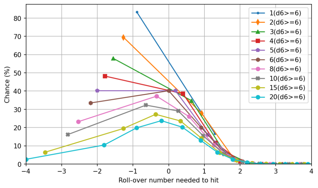
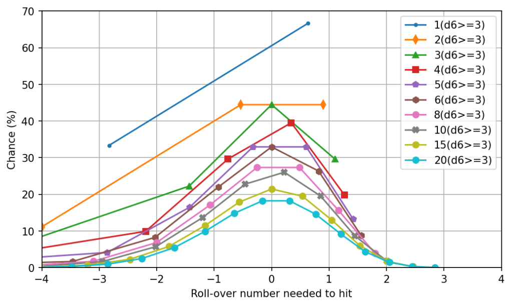


 . On the other hand, if in the corresponding fixed-die system both sides roll, the standard deviation increases by the same factor there. So overall we can expect a Gaussian still, just with a larger standard deviation and finer granularity by a factor
  , with the leftmost point in each series being
  .
. .
.
 dice to achieve the same. Here are some contributing factors:
 , the variance is
  , and the standard deviation is
  . 4+ on a d6 has
  . Using the formulas above, we find that
  , resulting in this table of correspondences:
 longer half-life than an individual geometric die. Since it requires a quadratic number of successes to keep up with a linear increase in the corresponding fixed-die DC, the argument to that falloff is now quadratic and the long tail becomes Gaussian-like in the fixed-die equivalent.

 and its standard deviation is
  .
. ), and still nearly half again as much as 2d10 (
 ). So in these cases, the clustering is mostly because of the smaller standard deviation rather than the inherent shape of the Gaussian.

 . This gives us the following PMF:

 producing a maximum absolute difference in chance to hit of 4.8%. That’s less than a single full face on a d20. This standard deviation is approximately equal to 3d12 (

 . Again, we’ll compare this to a Gaussian with the same standard deviation. First, the PMF:


 , then the mean and variance of their sum are


 is the chance of the die rolling a success when it doesn’t explode, then the mean and variance of the non-exploding part is:

 be the chance of the die not exploding and assume that each exploding face contributes one success directly. Then the mean and variance of the exploding part is:

 chance of success.

 . Therefore:

 and
and  respectively. The standard deviation is the square root of the variance, or
  .
.
 .
.

 , and the system is equivalent to a fixed-die roll-over system where the player is rolling a geometric die. In this case, the long tail favors the player.
 , since the die size increases by a factor of 10 every 10 steps, which is very close to doubling every 2 steps. d30, d40, d50, d60… can be easily rolled by using the lower part of the series for the tens place and a d10 for the ones place. For example, a d60 can be rolled using 1d6-1 for the tens place and 1d10 for the ones place.
 equals the number of dice in the dice pool.
 , which is slightly longer than
  but is the closest we can get with standard dice. Every die step above the TN is then about equal to one d10 in the pool. For example, a d16 is three steps above a TN of 8, which makes it similar to rolling three d10s looking for at least one 9+.
 .
.
 , out of which the area where
  . So the probability of


 that maps the number of dice
  that maps the number of dice
  , we can compose the two to find the mapping
  . In turn,
  , if we start at a particular to-hit number, an additional change to

 is the chance of failing on a single die. Let us take some more logarithms:

 ) becomes
  . If the dice pool is made out of d6s and we need a 6 to succeed,
  and
and  . So rolling 6d6 keep highest versus a TN of 6 is equal to a fixed-die system where we roll a die with a +7.8 bonus versus a DC of 5.8.


 .
. .
. close to zero, we can approximate


 and any such offset into a constant
  . This means that
 below:
 , or the “1” line above), one in 3.25 hits will have two successes, one in 15.01 hits will have three successes, and one in 89.91 hits will have four successes. Forged in the Dark operates mostly to the left of this line with respect to full and critical successes.
 rather than
  . The difference of bases translates to a constant offset in
  to vary continuously. Due to the granularity issues we looked at last time, any actual keep-highest dice pool system will not be continuous but rather discrete and uneven.
 . If we let
  then the chance of missing is
 . From here we have
  . If we used a target number of 6 instead, we would have
  .
. and
and  .
. would be a 25% miss chance,
  would be a 12.5% miss chance, and so forth.
 close to zero, we can again use a linear approximation:
 is proportional to

